CorrelScan Help
Introduction
CorrelScan is a general purpose correlation tool that
helps you compare all items in a list to all the others.
Most technical analysis programs that allow you to run such correlation scans, for example TCScan+, allow you to see how one
item compares to other items in a list. This is useful when you have a
particular item you are interested in, but if you are instead looking for good
trades within a basket of items, for example in pairs trading, then you need a tool
like CorrelScan.
The
primary statistical measure of how similar (correlated) two items are, is the
Correlation Coefficient. It can only have values from -1 to +1.
Values close to +1 indicate that the items behave very similarly, while values
close to -1 means they behave in an opposite manner. Values close to 0
indicate that the two items are not related at all. Examples are provided
below.
There
are a number of ways you can use CorrelScan:
 |
You can trade sets of similar
stocks off each other. If one stock starts a move, for example
after some good news, you can trade closely-correlated stocks to
it, knowing they will move in a similar way soon thereafter. If you played
the primary stock directly you might only catch the
tail-end of the move, whereas by buying its correlated
partners you could catch a much larger part of the
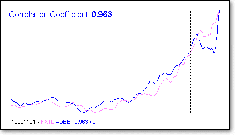
move. You would also lessen your risk by being more diversified. The chart below shows an example where two items are well
correlated up to the time of the scan (indicated by the vertical dotted
line) and then proceed to move the same after the scan date.
Notice that the two items do not move perfectly in sync either before or
after the scan date, but they generally follow the same direction - you
will always need to allow some margin of error in these types of trades. |

 |
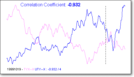
You can trade dissimilar stocks
off each other. If one starts trending up you can
short another that is anti-correlated to it knowing that there is a good
chance you will be right. The
chart below illustrates an example - note the continued dissimilarity
after the scan date. |

 |
You can balance your portfolio,
making sure that you have a diverse set of items that will not be affected by each other. In this
case you select items that are not
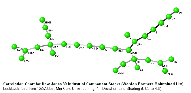
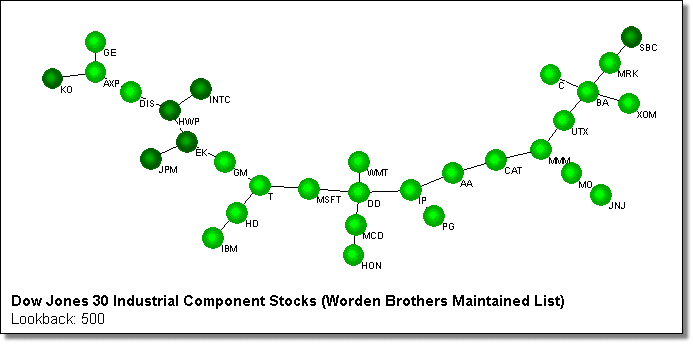
well-correlated with each other. The linkage chart below shows the
components of the Dow Jones Industrials list, with the most similar
items connected by lines. As described in more detail later, a
balanced portfolio should consist of items selected from the outer edges
of the chart, for example KO, HON, MSFT, JNJ and MMM in this example. |

 |
You can find items that normally behave very similarly, but are
currently not doing so. You can then take trades betting they
will soon revert to normal behavior - this is known as
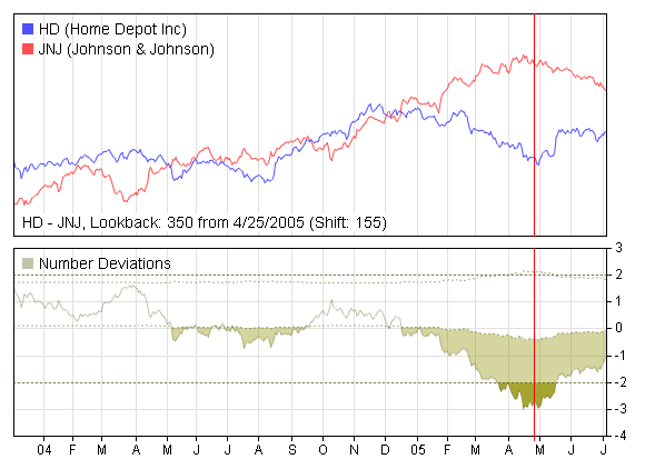
Pairs Trading (or more completely 'Risk Arbitrage Pairs Trading'.) An example chart is shown below. In the top
pane is shown the price data of the two items and in the bottom pane is
shown the relative price difference between the items (in terms of
multiples of the average difference between them.) You can see that the
items move more or less in sync until around February 2005, when they
start to diverge more than 'normal'. The scan date, indicated by
the vertical red line, is around May 2005 and this pair was highlighted
because the difference between the items was almost 3 times the normal
difference and the difference was starting to flatten out. This
behavior, for
normally well-correlated pairs, is an indicator that they may soon start
to revert to normal behavior. You can see that the items indeed
did turn around, so if you had shorted JNJ and bought HD (or their
options) you would have made a good profit. |

 |
You can find minimum volatility pairs, i.e., pairs where you take a long
position in one of the items and a short position in another so as to
reduce the volatility of your position. CorrelScan helps you to
balance the risk versus the return for the pair. The chart below
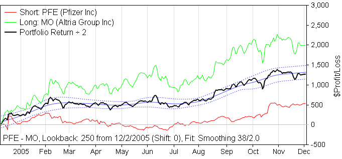
shows an example, where PFE was sold and MO was purchased. The
green and red curves show the trade profit for each item and the black
curve shows the average profit for the pair. You can see that if
you had just purchased MO, you would have made $4,000 profit, but would
have had to endure almost $1,500 changes in profit along the way.
On the other hand if you had just shorted PFE, you would only have made
$1,000 profit and had to endure $500 changes in profit along the way.
On the other hand, the combined pair would have made you $2,500 profit,
but more importantly, you would only have had to endure a maximum of
around $500 profit change along the way, with a much lower average
change than that. So you do not make as much as you could have -
but you sleep a lot more peacefully! |

Program Operation
|
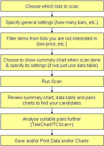
In
simple terms, follow these steps to run CorrelScan:
-
Select one or more lists from TeleChart to scan
-
Specify general program settings such as how many bars of data to include,
how far back to start the scan, whether to smooth the data, etc.
-
Specify list-filtering criteria to narrow down the items in the lists.
You can filter items based on price, range of movement, volume, exchange
type and optionability. This helps reduce the number of items in your
scan, which helps shorten execution time.
-
Specify whether a summary chart should be generated at the end of the scan
and provide settings for it. This chart is very useful for getting an
overview of how the items in your lists are related, but it can take a long
time to generate for large lists, so for these it may be best to disable its
generation and just use the output data table.
-
Run
the scan.
-
Review the summary chart (if it was generated) and/or review the data output
from the program. In both instances you are able to retrieve charts
and data for any of the pairs in your list (as shown in the introductory
examples above.) The data table allows you to sort and filter the
output by numerous criteria allowing you to find the potential trades you
want.
-
Save
and/or print the charts and/or data for later use.
These
steps are described in more detail below.
|
 |
Program Settings
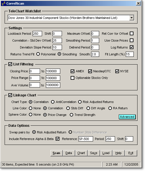
When first started, the main CorrelScan form will
appear similar to that shown below.

Each of the sections on this form are described below.
List Selection

At the top of the form you will see the list selection box.
All the lists contained in your version of TeleChart are there, including ones you have created yourself.
Be aware that
because CorrelScan compares every item in the list to every other item, the time
a scan takes is related to the square of the number of items. So for
example, a list with 70 items will take almost twice as long to scan as a list
with 50 items in it. This is not a prohibitive issue, because some users
regularly scan lists with 1,000 items or more in them, but when you are starting
out, we suggest you stick to smaller lists.
Settings

The
various general settings are as follows:
 |
Lookback
Period The number of days for which you want to correlate the
stocks against each other. Shorter periods will find short-term
trends and longer periods will find longer ones. We do not recommend
using periods below about 100 days, because such short correlation periods
are not likely to have continued relevance in the future. On the
other hand, the longer the lookback period, the longer it will take to
run the scan so you need to balance this setting. |
 |
Shift
The number of days back to start the scan. A value of '0' means
the scan will start with the most recent data. Increasing it allows you to
run scans for the past so you can evaluate how correlations at a certain point in time affected future
behavior. This helps you fine tune your settings so they suit your
requirements. |
 |
Maximum Offset is the maximum
amount of offset to be allowed in the search for the
best correlation. To clarify, consider two stocks 'A' and 'B' that
you are trying to correlate. CorrelScan will first work out the
correlation between 'A' and 'B' and will then shift 'A' both backwards and
forwards in time compared to 'B', one day at a time, until the maximum
number of days you specify in 'Max Offset'. At each point CorrelScan
will work out the new correlation, keeping track of the best one.
This best correlation is the one reported by CorrelScan, along with the
number of days of offset between the items when this correlation
occurred. This option is very useful, because changes in 'A' might lead
to changes in 'B' some days later, or vise versa. Knowing the best
correlation and offset period between 'A' and 'B' will allow you to
predict changes in 'B' based on earlier behavior in 'A'. The optimum
offset is included in the output data and if you choose to display the
linkage chart, it will also be displayed on the caption bar when you
move your cursor over the chart. If the offset
is shown as positive, then the base security
predicts the linked security, and if the offset is shown as negative
then the linked security predicts the base. |
 |
Ret Corr for Offset defines the method that will be used to find the
best offset between correlated items when you have a number entered for
the Maximum Offset. When this box is unchecked CorrelScan will
correlate the price of the two items in question. When it is
checked, the daily price change will instead be used. The former
favors longer-term/overall similarity, while the latter favors daily
responsiveness of one item to the other. You can ignore this
setting if you are not allowing the offset to be adjusted (which you
should do when starting out.) |
 |
Correlation - Std Dev Offset This setting is used mostly
for Pairs Trading, when you are looking for items that are normally
correlated but are currently not so, so you can trade them as they
revert to normal. CorrelScan works out the correlation for each
item as well as how far from normal the items currently are. The
problem, however, is that if the items have been away from normal for a
while, the correlation coefficient will be affected, because it will be
indicating to some extent the current disimilarity between the items
rather than how similar they normally are. Therefore it is useful
to only determine the correlation coefficient up to a certain point in
the past and remove any current divergence from the picture. The
number you enter in this setting dictates how many bars back the
correlation will stop. So, for example, if you enter '25' here and
your lookback period is 250, then the correlation will only be detemined
for the 225 days starting 25 days back. The most recent 25 days
will not be included in the correlation calculation. |
 |
Smoothing Period The value entered here will be used as the period for a simple moving
average of the data, which will then be used in place of the original data for the
correlation calculations. A smoothing period of 1 indicates the data
will be used unsmoothed. |
 |
Use Close Prices CorrelScan normally uses the average of the
open, high, low and close of each day for its calculations. If you
check this box it will only use the close price. |
 |
Deviation Slope Period This setting is also used
mostly for Pairs Trading. When CorrelScan calculates the deviation
between items, i.e., how different they currently are from normal, it
also works out the slope of the deviation. This helps you know
whether the difference between the items is increasing or decreasing.
The number entered in this setting is how much of the data to use to
work out the slope. For example a value of '10' means the last 10 days
will be used to work out the angle of the deviation. Higher
numbers are better for longer term positions and lower ones for shorter. |
 |
Price Change/Trend Period
is the time period over which CorrelScan should check whether the stocks
are trending or changing in price, for trend coloring (see above.)
|
 |
Detrend
Period
This setting allows you to remove the trend from the data, which is
sometimes useful to discover the underlying behavior between items.
We recommend, however that you leave it at 0 until you are more familiar
with the program. The number entered in this setting is used to
create a moving average of the data, which is then subtracted from the
data. This is a standard way to remove the trend from the data.
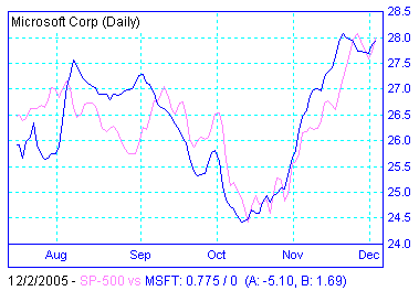
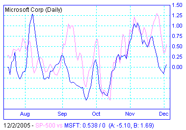
Shown below is a chart of MSFT compared with the SP-500 index, both with
and without 10 bar detrending. You can see in the latter chart
that the price action is flattened, emphasizing the relative movement of
the two items. |


 |
Log Returns
In a number of calculations, CorrelScan needs to determine the daily
change in price. This is also know as the return. This
return can either be calculated arithmetically, where the return is just
the price difference between the current day and the day before that
divided by the previous day's price. It can also be calculated
logarithmically, if you check the Log Returns box, in which case the
return will be calculated by the logarithm of the ratio between the
current and previous day's prices. The latter option is more
commonly used, especially in academic circles, though the results tend
to be fairly similar. |
 |
Returns Trend Fit / Smooth / Fit Length This setting is used when
finding minimum volatility pairs, that is, when you are trying to find
two items where you will go long one and short the other and you want
the overall volatility or risk of the position to be minimized.
This setting can be better understood after reading about this kind of
trade above, but in principle the daily return of the combined long and
short positions is plotted versus time and a curve is fitted to a
portion of the end of the returns curve to help calculate relevant
information about it. For example, it is important to know whether
the combined returns curve is increasing or decreasing, because that
indicates whether you would be winning or losing money in the position.
The type of curve fitted can either be a polynomial or smoothed.
If you choose the former you can specify the order of the polynomial - a
polynomial of order 1 is a straight line, order 2 is a parabola, etc.
If you choose the latter, you can specify the smoothness of the curve.
The 'Fit Length' specifies how many bars are used to calculate the
curve. |
List Filtering
Checking the List Filtering box will allow you to filter items in the selected lists by
price, volume, exchange and optionability. This is useful to reduce the
number of items in the list and speed up your scans.

 |
Closing Price allows you to select the range
of closing prices for items in your scan. |
 |
Price
Range allows you to select how much price movement the items in your
scan must
have had over the lookback period. CorrelScan searches all the data over
the lookback period, finds the highest and lowest prices and determines
the difference. This result must fall within the two numbers you enter.
Setting the range allows you to keep out very volatile or very range-bound
items. To ignore the price range, set the limits very wide, for example
from 0 to 100000. |
 |
Average
Volume allows you to select the average daily volume for your filtered
items. The value you enter is multiplied by 1,000 to get the actual
volume. Note that this is different from the TeleChart convention, which is
to show volumes divided by 100. |
Linkage Chart
Checking the Linkage Chart box will cause a chart to be generated at the end of
the scan. Other charts are available via the data grid and also via this
chart, but this one provides a good visual indicator of how items are correlated
with each other. The chart takes a long time to draw for large lists so
for these it would be better to not enable it and rather just use the data grid.
The linkage chart indicates correlation by drawing circles representing
each item, then draws lines linking the best correlated items together. It
allows you to quickly see which items are most like each other, and also those
which are least alike. An example is shown below for the Dow Jones Industrial
Components. You can quickly see that INTC and HWP are closely correlated for the
period of this scan, while SBC and KO are not. Full details and
settings for the linkage chart are described elsewhere
in this help file.

Data Options

This
section allows you to specify settings for the data table generated by the scan.
You can choose whether or not to swap the pairs in the table so the item to be
shorted is always in the first column and the long is in the second column.
You furthermore can choose whether to swap the pairs based on whether you are
trying to find minimum volatility pairs (Risk Adjusted Return option) or
long-short pairs trading opportunities (Number Stds Difference option.)
Note: the current beta version only allows the Risk Adjusted Return option - the
final version will allow all three.
The Data
Options section also allows you to specify whether you want to include reference
statistics for items in your list. If the Include Reference Alpha &
Beta option is checked, then CorrelScan will include
Alpha and Beta values for each item versus a
reference you specify.
Running
the Scan
After you have specified the above settings, press the
button marked Scan at the bottom of the main form to start the scan.
While the scan is running, the other buttons and settings boxes will be
disabled.
Before starting the actual correlation of items,
CorrelScan will first check if all the items in the list have sufficient data to
match the criteria you have specified. If not, it will ask if you either
want to delete the items that don't have enough data or change your settings.
After that the scan will run and progress will be shown on the status bar at the
bottom of the form. Since CorrelScan correlates all items in the list
against each other, you will see two progress bars - the first showing the
reference item at the time and the second the item it is being correlated
against. The scan will appear to speed up as it progresses, because an
item is not scanned again once it has been a reference (the correlation of A to
B is the same as for B to A.)
If at
any time you want to stop the scan, press the Scan button again, whose
caption will have been changed to Stop while the scan is running.
If you
have selected to show the linkage chart when the
scan is done, it will be generated automatically. While the chart is open,
the scan button will continue to be labeled Stop and the other buttons on
the main form will be disabled. Pressing the Stop button or closing
the linkage chart will allow access to the main form again, which will allow you
to review the data grid and access other functions. You can then save the current settings, data files and chart generation
data by clicking the Save button on the main form. This allows you
to
reload this data in the future by clicking the Load button. When
the data is reloaded all the data files created by the saved scan are copied
into your main CorrelScan directory, replacing those already there.
Likewise the chart data replaces that of your current scan, so you only need to
press the Chart button to view the chart, not rerun the whole scan.
Reviewing
Data
Once the
scan is complete and you have closed the linkage chart (if generated) you can
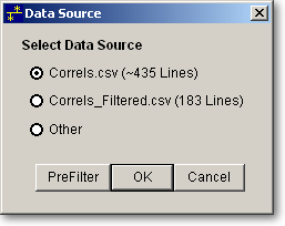
press the Data button to access the data grid. The first form you
see will allow you specify whether you want to view all the data or a subset of
it. You can also load another file that you may have saved previously.
For small lists you can just view all the data, but for very large lists (around
250 items or more) it is better to only view a subset of it. The full data
set is always called 'Correls.csv' and the subset is called 'Correls_Filtered.csv'.
Both are in your CorrelScan directory.

Data Filtering
The
subset file is created using a predefined set of filters to reduce the size of
the file. If you have not defined this previously or would like to change
the filtering criteria, then press the button marked PreFilter on the
bottom of the above form - this will open the Data Filter form.

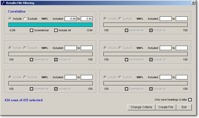
When
first opened, the form will only have one item you can filter by: Correlation.
To choose other items to filter by, press the button 'Change Criteria' at the
bottom of the form. This will allow you to specify up to a total of six
items whose range you can specify to filter out items you are not interested in.
To explain how the form functions, consider the portion of the above form for
the Correlation section:

At the
top left you see the name of the variable being filtered, in this case
'Correlation'. The blue bar in the center of the form allows you to move
the bounds of the filter range by clicking and dragging the edges with your
mouse. You can also set the ranges by entering numbers in the boxes (next
to 'Included:' above.) Checking the Include or Exclude buttons specifies
whether items inside or outside the select range will be included. As an
example see the form below with the left and right edges moved. You will
see that with the bounds where they are now, only items with correlations
between -0.41 and 0.73 will be included. The bold '69%' in the center of
the form means that only 69% of the data will be included, based on this filter.
You can also see from the numbers at the bottom left (-0.89) and right (0.94)
what the actual limits of the data are.

As
another example, shown below is the exact same form, but now with the Exclude
button checked. Here you see that all items with correlations between
-0.41 and 0.72 will be excluded. The '69%' does not change, but now
indicates what portion of data is excluded by this filter. The complete
count of items included by all the filters is updated at the bottom of the main
form.

Pressing
the Include All box will allow you to quickly remove the limits of this
variable in the filter. When the Symmetrical box is checked, the
left and right margins will be moved in equal amounts when the other margin is
moved.
As you
move the margins you will see the resulting number of rows displayed at the
bottom of the form. When you are satisfied with the reduced data set, you
must press the Create File button at the bottom right of the main form.
The settings that you have specified when you create this file will be used to
automatically filter your data the next time you run a scan, so you do not need
to go through this process every time unless you want to change the filtering
criteria.
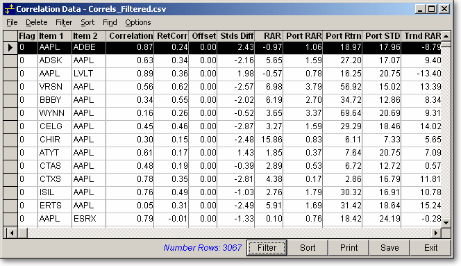
Data Grid
*** PLEASE NOTE: THIS
SECTION TO BE AMPLIFIED AND ELABORATED IN FINAL VERSION ***
Once you
have selected the data source and performed any prefiltering, the Data Grid will
be opened up.

The data
grid lists all variables generated by CorrelScan. You can choose which you
want to view, depending on what you are interested in, via the Options >
Hide/Unhide Columns menu. Likewise, you can choose which rows to
exclude (filter) by using the Filter menu. Clicking the heading of
a column will sort by that column and you can access sorts by multiple columns
via the Sort menu. The Delete menu acts differently from the
Filter menu. When you filter the data, it is just hidden from view,
and can be returned to view by changing your filter criteria (or selecting
Filter > Remove Filter.) When data is deleted, however, it is
removed from the data set and can not be returned unless you reload the data
again (which you can do via the File > Open menu or by closing the
form and reopening it again.) If you save the data (File > Save)
to the same file you loaded, you will not be able to retrieve the deleted data
except by running the scan again.
From the
Delete menu you can permanently remove items that are current filtered (Delete
> Filtered Items), delete all other rows (pairs) containing Item 1 or
Item 2 of the currently selected row or both. The Prune Pairs option uses
a combination of the preceding. It allows you to create a list where only
the top pairs are shown. For example, you can list all pairs that have the
highest correlation. It does this as follows: using your current sort
criteria, the pair at the top of the list will be selected. CorrelScan
will then delete all other pairs in the list containing either of the items in
this pair. It will then move to the next row and do the same, etc.
You will end up with a number of pairs equal to half the items in your list that
are ranked the highest according to your sort criteria and where no items are
repeated in any other rows.
To move
up and down the data grid, you can press the Space/Backspace keys or
click the selector bar at the far left of the columns. To select multiple
rows you can hold down the Shift key and click on the selector bar for
the first and last row of interest. Likewise, use the Ctrl key to
select non-contiguous rows. When items are selected you can flag them via
the right-click menu. Flagging works by increasing or decreasing the count
in the column headed Flag. From the right-click menu you can
increment, decrement or zero the flag. You can then use this column as
part of your sort or filter criteria.
When the
data grid is opened the pairs chart will be opened automatically and will be
changed as you navigate through the pairs. You can switch between
Deviation Mode and Non-Deviation mode via
the chart's Option menu.
A
summary of the variables and column names available in CorrelScan for the
various scan types is listed
below. (Further details, formulae and examples will be
included in the final version.)
Correlation
Scan
|
Flag |
A counter that you can
increment and decrement via the right-click menu and then use in your
sort and filter criteria |
|
Item 1 / 2 |
Name of 1st/2nd item in
pair |
|
Correlation |
The correlation
coefficient for the pair |
|
RetCorr |
The correlation
coefficient for the daily
returns of the pair, rather than the absolute price |
|
Offset |
The offset at which the
correlation (or returns correlation) is maximum. You can specify
the maximum offset to check on the main form under 'More Options' (This
feature not fully debugged in the current Beta) |
| RAR |
The Risk Adjusted Return
of the pair, defined as alpha
divided by the standard error. |
| Price 1 / 2 |
Current price of items 1 and 2 |
| Alpha, Beta, Std Err |
See a full description
here. |
| RefAlpha, RefBeta,
RefStdErr |
Alpha, Beta and Standard error of the
item versus the reference you specify on the
main form. |
| Item Industry/Sub
Industry |
The Industry (sector) and SubIndustry (subsector)
for item 1 and 2. These follow the Worden classification within
TeleChart |
| AbsCorr, AbsRetCorr, etc. |
These are absolute values of the
equivalent variables defined above. They are included to help in
sorting & filtering where you do not care about the sign of the
variable. |
When
running correlation offset calcs (i.e. seeing at what relative offset between two
items the correlation is highest), the following additional fields are
shown:
|
C_Offset |
Optimum offset between the two items -
if this number is at the maximum offset you specified then it is not
meaningful |
|
C_Corr |
Correlation value at the optimum offset |
|
C_RetCorr |
Returns correlation value at the optimum
offset |
|
C_dCorr |
Difference between the non-offset
(normal) and offset correlation values |
|
C_dRetCorr |
Difference between the non-offset
(normal) and offset returns correlation values |
|
R_Offset, R_Corr, R_RetCorr, R_dCorr,
R_dRetCorr |
These are equivalent to the above items,
but in this case the information is provided for the optimum offset
based on highest returns correlation rather than highest price
correlation |
Risk Arbitrage Pairs
Scan
In
addition to the above items, the ones in the table below are also shown for this scan type.
Many of these relate to the spread (i.e. difference in price) between the two
items in question, which is an indication of how the two items move in relation
to each other over time. The spread is the main line shown on the lower part of the
chart when you click on a pair in the data table. Note that this scan type
is not valid for items with low correlations (roughly less than 0.5), so it is
best to filter these out using the 'Prefilter' option when the data file is
opened. Note also that this scan type includes estimates of back-tested
profitability over the scan period. To calculate this, CorrelScan
estimates optimum upper and lower cut points for the spread curve. When
the spread curve passes down through the upper cut line or up through the lower
cut line a trade is entered by shorting one item and buying the other. When the spread curve crosses the opposite
cut line the trade is closed. Information on individual trades taken can
be seen by clicking the 'Trades' menu item on the chart. Also see the picture below for further
clarification of terms.
For more details on this scan type, refer to 'Pairs Trading: Quantitative
Methods and Analysis by Ganapathy Vidyamurthy'.

| Crosses |
The number of crosses that the spread
curve makes through the zero point, which is an indication of how
mean-reverting the spread curve is, i.e., how likely it is that the
spread curve will revert to equilibrium (and that the items in question
will oscillate around each other.) |
| DaysCrs |
Average number of days between crosses
(see above) |
| Stat1/Stat2 |
These will be explained in further
detail in the final program version - they are different measures of
Stationarity, i.e., how likely it is that the spread curve oscillates
regularly. The higher these statistics the higher the level of
stationarity / mean reversion / crosses. |
| Trds/Yr |
Number of trades per year |
| %Profit |
Total percentage profit for all trades
(Click the 'Trades' menu item on the chart to see info on individual
trades) |
| %MAE |
Maximum adverse excursion as a
percentage of dollars invested (for example if $1,000 is invested and
the furthest a trade goes against you before it closes is $250, then the
%MAE is 25%.) An example of how the trade can go against you is
shown in the above chart between July and August - the trade is entered
at the lower cut line at the start of July and then instead of the
spread curve proceeding directly to the upper cut line, it meanders
around and even goes significantly lower than the lower cut line,
causing a negative position, before finally heading to the upper cut
line around 10 August. |
| TrdDays |
Days spent in-Trade |
| %LossDays |
Percentage of days in trade that are
losing days |
| Slope / Intcpt |
Slope and intercept used for calculating
the spread curve: Spread = Item 2 Price - (Item 1 Price * Slope +
Intercept) |
| Cut_L / Cut_U |
The 'optimum' cut points for determining
the extremes of the spread curve - see introduction to this section |
| MAE_10%/2% |
To be described later |
Minimum Volatility Pairs
Scan
In
addition to the above items, the following are also shown for this scan type.
Many of these relate to the spread (i.e. difference in price) between the two
items in question, which is an indication of how the two
| Port RAR |
The minimum variance risk adjusted
return for the portfolio. This is the risk adjusted return for the
pair at the point on the return versus standard deviation chart where
standard deviation is a minimum (the minimum variance point.) |
| Port RTRN |
The return value at the minimum variance
point. |
| Port STD |
The return standard deviation at the
minimum variance point. |
| Trnd RAR, Trnd Slope,
Trnd Err |
A line or polynomial is fitted to the
latter portion of the average profit curve for the pair. The Trnd
RAR is the slope of the line (Trnd Slope) divided by the standard error
(Trnd Err.) |
| MeanPrice 1 / 2 |
The expected price of Items 1 and 2,
based on predictions from the normal difference between the two items.
These numbers only have relevance for normally well correlated (or
anticorrelated) pairs. |
| Pct Gain |
The potential percentage gain from
taking a short/long position in Item 1/Item 2. This is based on
these items returning to their MeanPrice and is only relevant for items
that are normally well correlated. |
| Dev Angle |
The slope of the relative difference
curve for the pair. When the Stds Diff is high, you can look for a
flattening slope to indicate that a retracement is imminent. |
| RetMean1/2 |
Average return for items 1 or 2 |
| RetStd1/2 |
Standard deviation of returns for items
1 or 2 |
FURTHER INFORMATION,
EXAMPLES AND METHODS TO BE INCLUDED IN FINAL VERSION
